When you do use the Pearson correlation coefficient, always test for significance. But don’t use it to analyze time series. It’s a common mistake. It violates the independence of observations and ignores the relationship between lags. Instead, use cross-correlogram analysis to identify relationships between time series, including lagged relationships.
“All models are wrong, but some are useful” is a recurring phrase among those who practice statistics. It originates from a statement by George Box, one of the great statisticians of the 20th century: “Since all models are wrong the scientist must be alert to what is importantly wrong.” (Box 1976). “All models are wrong”, means that models are instrinsically limited and will not perfectly capture reality. In other words, a model is a simplified representation of reality, used to explain or predict a phenomenon. If it were a perfect explanation of this phenomenon, it would cease to be a model and become a law.
In statistics, we essentially deal with random or stochastic variables, that is, variables that have a probability distribution (Gujarati and Porter 2021). Our mission as analysts is to develop and utilize methods that tell us how to formulate functions allowing us to describe and predict the relationship between these variables, while minimizing stochastic errors.
Depending on the functional form and the chosen estimation method, there are a series of assumptions that must be met for any inference about the error, coefficients, predictors, and regressands to be valid. If these assumptions are ignored, there is no guarantee that the results found are an optimal approximation of the function one aims to estimate. Not only that, but the violation of some of these assumptions can generate misleading results, showing significant statistical relationships where none should exist, underestimating or overestimating the object of study.
In this post, I address some frequent methodological errors that cause some models to be useless.
1 LET’S GET SOME DATA
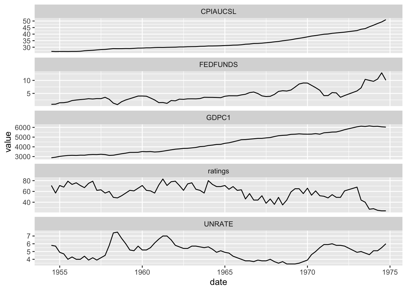
Have you ever heard about presidents dataset? From the built-in {datasets}, it stores US presidents quarterly approval ratings from 1945 to 1974. Does it hold any relationship with consumer price index (CPI), real GDP, unemployment rate or interest rates? Let’s find out!
# convert to dataframepresi <-data.frame(date = zoo::as.Date(zoo::as.yearqtr(time(presidents))),ratings =as.vector(presidents)) |>na.omit()# get CPI and funds rates from FREDquantmod::getSymbols(c("CPIAUCSL", "FEDFUNDS", "GDPC1", "UNRATE"),src ="FRED")
[1] "CPIAUCSL" "FEDFUNDS" "GDPC1" "UNRATE"
# convert to time seriesseries <-lapply(list(CPIAUCSL, FEDFUNDS, GDPC1, UNRATE), function(serie) {# serie name serie_name <-names(serie)# convert to dataframedata.frame(date = zoo::as.Date(zoo::as.yearmon(time(serie))),value =as.vector(serie) ) |>setNames(c("date", serie_name))})# merge datasetspresi_merged <-Reduce(function(x, y) merge(x, y, by ="date"),c(list(presi), series))# visualizekbl(head(presi_merged), booktabs =TRUE, digits =2) |>kable_styling(latex_options =c("striped", "scale_down"))
The first, and often only, resource for variable selection and model specification among those not initiated in time series analysis is the Pearson correlation coefficient \(r\). If we try to use it, we’ll’ have the following results (Table 2):
According to the rule of thumb for interpreting the effect size of the Pearson correlation coefficient1, CPI, interest rates and GDP have all large correlation with presidential approval ratings, while unemployment rate has small correlation.
Even if it were appropriate to use the Pearson correlation coefficient to select variables, a test must be performed to verify if the found coefficient is statistically significant. In this case, we can verify that the 10% correlation between presidential approval and unemployment rate is not significant. Ignoring significance tests results in erroneous interpretation, leading the analyst to find relationships where, in fact, none exist.
When it comes to inferential statistics, making any statement requires performing hypothesis tests. Except in extreme cases that prevent the estimation of some coefficient, in most cases, it is possible to obtain some statistical measure, such as in regressions, analysis of variance, correlations, etc. However, obtaining a number does not mean it is valid or can be used.
The correlation coefficient calculated from a sample (\(r\)) is a point estimate of a population parameter (\(\rho\)). Like any sample-based estimate, it has sampling variability and, therefore, must be accompanied by a confidence interval (CI) that reflects the uncertainty of this estimate and provides a range of plausible values for the true population parameter. This value \(r\) is a central point (mean) around which the confidence interval for the true value is constructed.
If, due to sampling variability, \(0 \in CI\) (e.g., \(r=0.05\) with a confidence interval of \([-0.01,0.11]\)), then there is no statistical evidence to claim that the mean value of 0.05 is different from zero.
3 ERROR #2: USING THE PEARSON CORRELATION COEFFICIENT
In section Section 2, I said “even if it were appropriate,” because it is not. The Pearson correlation is inadequate for assessing the correlation between two time series because it violates fundamental assumptions of the Pearson coefficient.
First, it violates the independence of observations. One of the assumptions of \(r\) is the independence of observations within each variable and between variables. Time series, by nature, usually exhibit autocorrelation, that is, an observation \(y_t\) is correlated with \(y_{t-1}, y_{t-2}, \ldots, y_{t-n}\).
Second, it ignores the relationship between lags. The correlation between two time series \(y_t\) and \(z_t\) may not be contemporaneous. One series may influence the other with some delay (e.g., \(y_t\) correlated with \(z_{t-3}\) but not with \(z_t\)). The Pearson correlation only measures the linear relationship at the same point in time, ignoring these lagged relationships.
There are some valid ways to identify the relationship between two time series. One of the simplest is the cross-correlogram analysis. It allows you to identify not only the contemporaneous relationship but also the relationship at each lag of the time series.
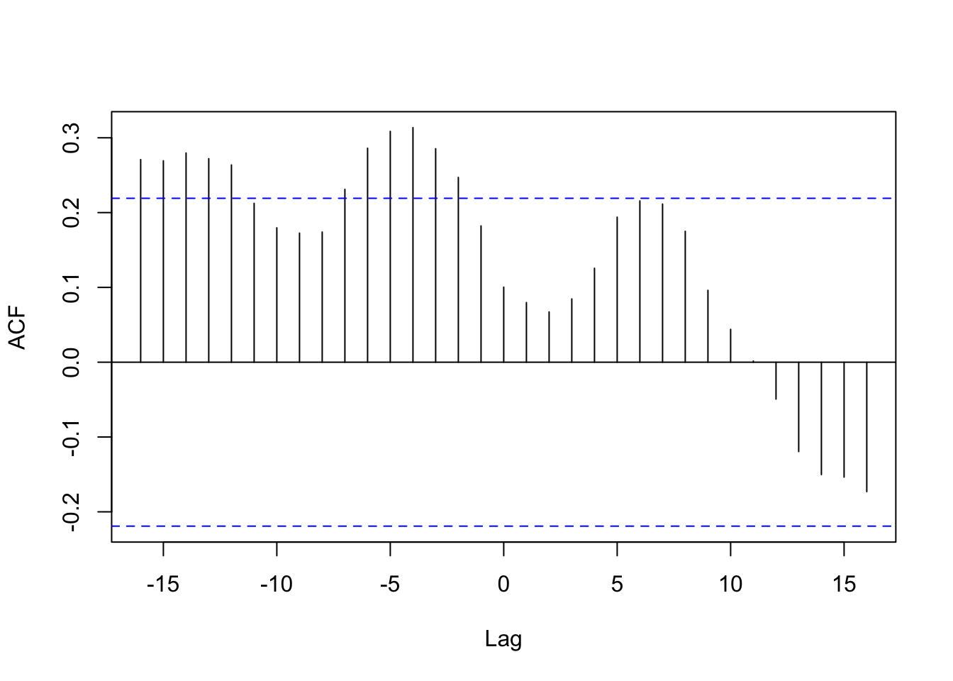
Now let’s look at the cross-correlogram between the time series of unemployment rate and presidential approval ratings:
Figure 2: Cross-correlogram between unemployment rate and presidential approval ratings.
If it were appropriate to analyze the two time series directly, we would see that, although there is no significant contemporaneous correlation — as we see by the correlation within the confidence interval at lag 0 —, they appear from \(t-2\), which would mean that unemployment rate from 2 months ago impacts the current presidential approval ratings.
References
Box, George Edard Pelham. 1976. “Science and Statistics.”Journal of the American Statistical Association 71 (356): 791–99.